Objectives
This tutorial is meant to introduce pomodoro package only, using a case study. The purpose of this package is modelling and reporting the predictive modelling with ease.
Dataset
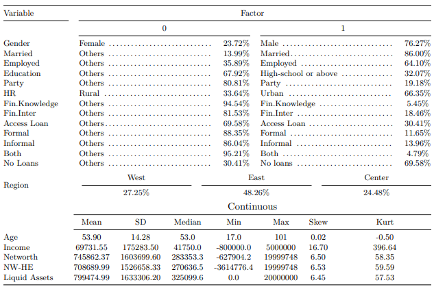
After cleaning the data set for this case study, we can visualize the summary statistics of the given data.

Note: HR stands for Household Registration. NW-HE is net-worth minus home equity. All the asset variables (e.g. income, net-worth, NW-HE, and liquid assets are in Chinese renminbi (CNY).
Overview
Package pomodoro runs currently bagging
(BAG_Model), boosting (GBM_Model), random
forest (RF_Model), multinominal logistic
(MLM_Model), and logistic models (GLM_Model).
This package is useful when you need the compare the predictive modeling
using the different data splits or/and adding exogenous variables into
the equation. And it divides the data set into 80/20 train/test set,
using stratified random sampling and implements 10 cross validation to
each model.
Installation
You can install pomodoro from CRAN with:
Building a Selected Model
Let’s build RF_Model one of the models which is
available for this package. In the pomodoro help
field we can see that RF_Model was defined as
RF_Model(Data, xvar, yvar).
DataSet
For the computational purposes lets take the first 1000 rows of the
sample_data.
Selecting Dependent Variables
where xvar is a vector which is defined as below:
Selecting Independent Variables
where yvar is a two or multilevel factor variable which
is defined as below:
or
Implemantation
We can implement RF_Model for
yvar <- c("multi.level") as follows,
Results of the RF_Model
Using attributes(BchMk.RF), we can see the outcome
options.
BchMk.RF$results
  mtry  Accuracy     Kappa AccuracySD    KappaSD
1    2 0.7640207 0.1712487 0.01929120 0.06294866
2    6 0.7288629 0.1729132 0.06145650 0.15118984
3   11 0.7264250 0.1782029 0.03964603 0.11603731
head(BchMk.RF$Pred_prob)
BchMk.RF$Roc
Call:
multiclass.roc.default(response = Y.test, predictor = Pred.prob)

Data: multivariate predictor Pred.prob with 2 levels of Y.test: zero, one.
Multi-class area under the curve: 0.7143
BchMk.RF$ConfMat
BchMk.RF$ACC
Building an Estimated Models
To model all the data set and its splits, interchangeably with 3
assets owning variables
(networth, networth_homequity, and liquid.assets) and given
an exogenous variable, in this case
exog = "political.afl".
Let’s build RF_Model again but this time . In the
pomodoro help
field we can see that Estimate_Models was defined as
Estimate_Models(DataSet = Data, yvar, exog = NULL, xvec = xvar, xadd, type, dnames).
We have already defined xvar, yvar and
Data.
Selecting exog Variable
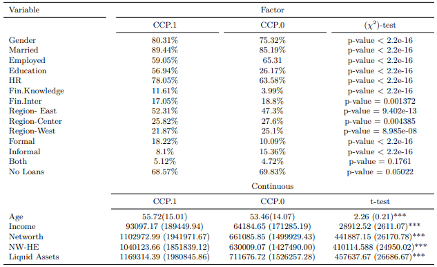
exog = "political.afl" will define the data set based on
the factor levels of the "political.afl" in this case “0”
and “1”.

Note: HR stands for Household Registration. NW-HE is net-worth minus home equity. All the asset variables (e.g. income, net-worth, NW-HE, and liquid assets are in Chinese renminbi (CNY).
Selecting xadd Variable
xadd is a vector set which are not highly correlated
with "income" but highly correlated between them. So we
need to add each variable in
xadd = c("networth", "networth_homequity", "liquid.assets")
interchangeably.
Selecting type Variable
type can be on of the bagging (BAG),
boosting (GBM), random forest (RF),
multinominal logistic (MLM), and logistic models
(GLM).
Selecting dnames Variable
dnames is the factor values of exog. For
example dnames = c("0","1") since there are 2 levels in
exog = "political.afl" which is “0” and “1”.
dnames argument is important to avoid confusion when we
print out the results.
Implemantation
We can implement Estimate_Models for
yvar <- c("multi.level") as follows,
Results of the Estimate_Models
Using CCP.RF, we can see the outcomes of
BchMk+networth, BchMk+networth_homequity,
BchMk+liquid.assets D.0+networth,
D.0+networth_homequity, D.0+liquid.assets,
D.1+networth, D.1+networth_homequity, and
D.1+liquid.assets.
Estimate_Models implemented RF_Model,
firstly to all data set as it is called BchMk, secondly
D.0 and lastly D.1, adding 3 asset variables
interchangeably.
Where D.0 and D.1 are coming from the
dnames = c("0","1") and can be interpreted as
D.0 when political.afl == 0 and
D.1 when political.afl == 1
Estimate_Models reported BchMk with all the
exog variables and divided all the data set
(BchMk) in to 2-level, when the observation has
political.afl == 0 or political.afl == 1,
Since this is a list object we need to use attributes as
follows,
> CCP.RF$EstMdl$`D.1+liquid.assets`$results
  mtry  Accuracy     Kappa AccuracySD   KappaSD
1    2 0.7926901 0.3348631 0.04543311 0.1835925
2    6 0.7929825 0.3707344 0.03656725 0.1258099
3   11 0.7979532 0.3894589 0.03274767 0.1245565
> head(CCP.RF$EstMdl$`D.1+liquid.assets`$Pred_prob)
zero one
3 0.992 0.008
4 0.124 0.876
8 0.290 0.710
25 0.742 0.258
33 0.854 0.146
36 0.750 0.250Building a Combined Performance
Estimate_Models reported predictive results for both
political.afl == 0 and political.afl == 1.
What we need is to combine these split data set to calculate over all
the performance for the political affiliation data split.
In the pomodoro help
field we can see that Combined_Performance was defined
as Combined_Performance(Sub.Est.Mdls).
We have already defined all we need in Estimate_Models
let`s bring them together.
Implemantation
Results of the Combined_Performance
Using attributes(CCP.NoCCP.RF) we can see the outcomes
of Combined_Performance
head(CCP.NoCCP.RF$Pred_prob)
CCP.NoCCP.RF$Roc
Call:
multiclass.roc.default(response = Combine.Mdl$Actual, predictor = Pred_prob)

Data: multivariate predictor Pred_prob with 2 levels of Combine.Mdl$Actual: zero, one.
Multi-class area under the curve: 0.6929
CCP.NoCCP.RF$ConfMat
CCP.NoCCP.RF$ACC
Have Fun!